Analysis
Analysis
The DCS Cloud Analysis is an online collaborative analysis tool based on Jupyter. It aims to help users easily create, organize, and share project code, data, environments, and results while ensuring reproducibility. It supports both online and offline analysis.
Online Analysis
Online analysis is a collaborative analysis tool based on Jupyter.
Quick Start for Online Analysis
Before running an online analysis, you need to complete the following steps:
Create a Project
The first step to analyze on the DCS Cloud is to create a project on the "Project Management" home page. Alternatively, you can analyze within a project you have joined.
Build an Image
An image is the basis for starting an analysis container and includes a complete file system, runtime environment, and necessary dependencies. By using an image, you can create one or more containers, each being an independent running instance. Create a custom image in the project's Image module.
Prepare Data
Container file mounting associates project files or directories with the file system inside a Docker container, allowing the container to access project files. By mounting files, you can read project files from within the container. Upload data through Data and mount the files from Data into the starting container. You can also directly mount the analysis result data from Data.
Run Analysis
Click the "Quick Run" button in the upper right corner to start the analysis container and begin the analysis.

Tips
The system will default to 1 core and 4G of computing resources and the default analysis image for the first quick run;
For subsequent runs, the system will use the most recently selected resource configuration and image to start the analysis container.
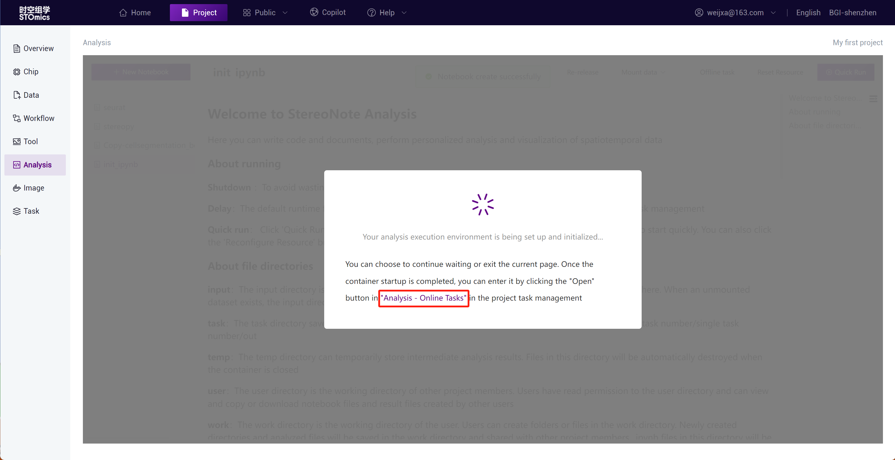
If the image resource is too large, the analysis container may take a long time to start. You can click on "Data Analysis ‑ Online Tasks" on the startup prompt page to jump to the "Task Management" module's "Data Analysis ‑ Online Tasks" section.
Once the container has started, click the "Open" button on the operation bar to enter the container directly.

Introduction to JupyterLab

The main elements of JupyterLab are:
Left Sidebar, supporting the following functions:
a.View and manage files created or added (uploaded or downloaded) during analysis, including .ipynb files;
b.Manage current kernel sessions;
c.Display the structure and contents of the currently opened .ipynb files, supporting quick browsing and jumping;
d.Install, uninstall, enable, and disable JupyterLab extensions to enhance and customize the functionality of JupyterLab.
File Directory
input: Data mount directory;
output:The output directory is used to store files that you want to save to the project's data management. After the analysis container is closed, all files will be directly uploaded to your project files for analysis by other project members. Please note that resetting resources and mounting data will launch a new analysis container and trigger data saving.
task: View the results of offline analyses that have been run;
temp: Intermediate analysis results can be temporarily stored in this directory; files in this directory will be automatically destroyed after the container is closed;
users: View other project members' .ipynb files and offline analysis task results;
work: Working directory where users can create folders or files. Newly created directories and analysis files will be saved in the working directory and shared with other project members. The .ipynb files in this directory will be read by the system and displayed on the "Personality Analysis" module homepage. .ipynb files in deeper directories under the work directory will not be read.
Toolbar, providing common functions and operations such as saving files, cutting, copying, and pasting code blocks, undoing and redoing, running, interrupting the kernel, restarting the kernel, et cetera.
Notebook, containing interactive analysis code and output results, along with associated Markdown comments.
Cell, where you can enter code, Markdown, and raw text.
Terminal, a JupyterLab terminal extension, similar to Linux shell or Windows Power Shell.
Console, providing an interactive command‑line interface that allows you to execute commands and operations within the JupyterLab environment, facilitating experimentation, debugging, and data processing.
Container Control
Save Environment: Supports saving the current running container environment as a new image;
Reset Resources: If the resources used during analysis are insufficient or you need to switch image environments, you can reapply for analysis resources and switch images by "Reset Resources". The container will restart with the configured resources;You can also change the resource configuration before starting the analysis.

Note
You can choose to build an image by "preset image" or directly save the container environment. Currently, images built by "Import from external sources" are not supported.
Mount Data: Modify the data mounts of the container. The user‑mounted data will be in the container input directory. Supports file mounting and analysis task mounting.
File Mounting: Supports mounting data from the project's "Data Management" module;
Tips: File mounting supports a maximum of 1000 files.
Task Mounting: You can mount any task's result data from the project or quickly select the first 1000 task result data in reverse chronological order for mounting.
Note
Task mounting supports a maximum of 1000 tasks.
You can also mount data before starting the analysis.

Note
If no data is selected for mounting before starting the analysis, the system will default to mounting the first 1000 tasks' result data from the project when the container starts.
Close: Close the container, stop the analysis;
Delay: Extend the analysis duration;
Save Data
When the container is started, an output directory will be automatically generated. The result data that needs to be synchronized to the project "Data Management" should be copied to the output directory:

Step1: Launch Terminal

Step2: Use commands to move or copy the file to the output directory

Examples:
- To move the 1.md file from the work directory to the output directory, you can use the following command:
mv /data/work/1.md /data/output/
- To copy the 1.md file from the work directory to the output directory, you can use the following command:
cp /data/work/1.md /data/output/
Step3: After completing the analysis and transferring all data to the output directory, close the container. The files in the output will be automatically uploaded to the "Data Management"/Files/ResultData/Notebook/{user}/output/{project_id}/ directory.

Note
When the container is closed, the data in the output directory will be automatically uploaded to "Data Management". Mounting data and resetting resources will restart the container, which also triggers the automatic upload of data.
The status of the saved data can be viewed in the "Task Management-Data Analysis" module.

AI-Assisted Programming
Stereonote-AI is an auxiliary programming plugin developed by the Time and Space Cloud platform based on Jupyter-AI and combined with the platform’s self-developed Genpilot. It aims to improve the efficiency and productivity of data work. You only need to ask questions in plain and simple language, and Stereonote-AI will write or modify code according to your instructions. It can also provide clear explanations for complex code to deepen your understanding. Whether you are an expert or a beginner in coding, Stereonote-AI can help you complete programming tasks excellently.
::: Stereonote-AI is only available in the Alibaba Cloud region. ::: ::: Stereonote-AI utilizes generative AI technology based on large language models (LLMs) to provide answers based on your instructions. The generated outputs such as code and text can include errors, biases and inaccuracies. Please always review code before running it. ::: ::: You can use stereonote-ai as a base image to install the required software packages and build a custom image with an AI assistant. For details on how to build a custom image based on the base image, see Building on the Platform's Preset Base Image. :::
Stereonote-AI is encapsulated in the official image stereonote-ai. Select the stereonote-ai image to start the container and experience the related functions:

Stereonote-ai offers two different user interfaces. In JupyterLab, you can use the chat interface to converse and help process the code. Additionally, you can invoke the model using the %%ai magic command.
Programming Assistant
The Jupyter chat interface is shown in the figure below, where users can directly converse with Jupyternaut (the programming assistant).

Simple Q&A:

Code Generation:
Enter the question directly in the dialog box.

Code Explanation:


Code Rewrite:
If you are not satisfied with the code, you can also ask to rewrite the code:

Code has been rewritten:

Notebook File Generation:
You can generate a notebook directly using the /generate command:

You can view the AI-generated Notebook files in the /data/work directory:

Magic Commands
Use %ai and %%ai as magic commands to invoke the AI model; you need to load the magic commands first:
%load_ext jupyter_ai_magics
View instructions for use:
%ai help
Basic syntax for the ai magic command
The %%ai command allows you to invoke the selected language model using a given prompt. Its syntax is :, where can be understood as the model provider, such as huggingface, openai, and is a specific model from the model supplier. The code block starts with the prompt from the second line.
The official model provided by DCS Cloud is: stereonote_provider:depl-gpt35t-16k. To invoke it, you need to use:
%%ai stereonote_provider:depl-gpt35t-16k
Code Generation:
We change the parameter of format to 'code' and select a difficult problem on the LeetCode platform with a pass rate of 30.7% for AI to solve.

The generated result code is as follows:

It passed directly after submission on LeetCode.

Simple Volcano Plot Drawing:

Generate results and run:

Code Debug:
We find a Python code snippet containing five errors:
    def calcualte_area(radius):
      if type(radius) =! int or type(radius) != float:
          return"Error: Radius should be a number.
      else:
          area = 3.14 * raduis**2
      return area
    print calcualte_area('5')
Let AI correct it and explain the reasons:

Not Limited to Programming:
Apart from code-related functions, AI can also generate LaTeX formulas, web pages, SVG graphics, etc.
LaTeX Formulas:
We want it to generate the Bernoulli equations. Just change the parameter of format to 'math', and the result will be output in LaTeX formatted style.

Web Page:
We let it generate a login page, where the format parameter needs to be changed to 'html'.

SVG Graphics:
Let AI directly generate some simple graphics for display in SVG format.

How to Clone Notebook Files Across Projects?
To quickly reuse code in other projects, the Temporal Cloud platform supports cloning Notebook files (.ipynb files) into the target project.
Step1: Select the Notebook file (.ipynb file) you want to clone and click the "Clone" button;Step2: Enter the name for the Notebook file after copying to the new project, select the target project to clone into, and click confirm. The Notebook file will be cloned into the target project.

How to Publish Notebook Files to the Public Repository?
The public repository is the developer ecosystem community of the Temporal Cloud platform, offering content sharing of images, data, applications, and workflows. It provides a secure, open asset sharing and usage to accelerate the development and implementation of applications, ensuring efficient realization of commercial value for all participants in the development ecosystem chain.
Users can publish high‑quality Notebook files to the public repository. Notebook files can also be copied from the public repository to projects for analysis.
Add File Tags and Description
Before publishing to the public repository, you can add a description and tags to the file for quick identification and filtering. Click "Edit" to add a description and tags.

Publish to Public Repository
Select a file or folder and click "Publish." Currently, individual files and folders can be published:

Individual File Publish: After publishing to the public repository, it will exist as an "Application";Individual Folder Publish: Publishing to the public repository will exist as an "Application Toolbox." The public repository "Application Toolbox" is a collection of analysis methods, and users can directly copy the "Application Toolbox" to the project to reproduce results;
Note
Only Notebook files in the current directory are supported for publishing;
The description and tags filled in during the publishing process will be published as the description and tags of the application toolbox.
Revoke Publication, Republish
After publishing the Notebook file, you can view and search for the published Notebook in the public repository. Published Notebook files can also be "revoked" or "republished."

How to Copy Public Repository Notebook Files to a Project?
Add Notebook files from the public repository "Public Applications" to your own project. Click the "Copy" button.

Select the target project. Only projects created or managed by the user are supported for copying.

Offline Analysis
If your data processing requires a long duration of continuous running, it is recommended to use "Offline Tasks" for cloud‑hosted running: the platform will run the entire project for you, and you can also view the running results, resource usage, and system logs in real time.
Quick Start for Offline Analysis Tasks
Task Creation
In the "Personality Analysis" module, click the "Offline Analysis" button.

Parameter Configuration
The default "Task Type" is Notebook; click "Select Notebook"

Select the already created Notebook file and "Confirm."

Creating offline tasks with a Notebook file supports three ways of parameter configuration:
- No Parameters: Default run the selected Notebook file code, creating one offline task.

- Adding Parameters: Manually add parameter groups on the page; multiple parameter groups can be added. Each group of parameters will create one offline analysis task.

- Parameter File Configuration: Download the json or Excel template, fill it out, and import it. Each group of parameters will create one offline analysis task.

Below is an example of parameters for creating batch offline analysis tasks using the json template method:

Below is an example of parameters for creating batch offline analysis tasks using the Excel template method:

Resource Configuration
Select the computing resources and image resources needed to run the task.

Deliver the Task
Click "Run" to deliver the analysis task.

Process Monitoring
After the offline task has been delivered, you can view it in the "Task Management ‑ Data Analysis" offline analysis module. Click "Open" in the task bar to view the offline task running status.

Click the "Details" button on the operation bar to view task details, task logs, and resource consumption.


Creating Offline Analysis Tasks Using a Script
Create a Script and Copy its Address
Create a script during online analysis.

Right‑click on the script file and select "Copy path" to copy the file path.

Parameter Configuration
When running an offline task, select "Run Script" as the "Task Type" and enter the run command. A set of instructions will create an analysis task.

Note
The path of the script file copied inside the container needs to be prefixed with the root path /data when running:
Copied path: /work/test.py
When running the script, use the path: /data/work/test.py
Resource Configuration
Select the computing resources and image needed to run the task.

Deliver the Task
Click "Run" to deliver the analysis task.

Process Monitoring
After the offline task has been delivered, you can view it in the "Task Management ‑ Data Analysis" offline analysis module. Click "Open" in the task bar to view the offline task running status.
